Time Series

A time series refers to a collection of data points that are observed or measured over a sequence of time intervals. It consists of a series of observations or measurements taken at different time points, with each data point associated with a specific time stamp.

Time series modeling is a way to understand and predict patterns in data that change over time. Time series modeling helps you analyze this data to uncover trends, patterns, and relationships between past and future values. With time series modeling, you can make predictions about future values based on the historical data you have. It’s like looking at the past behavior of something to make an educated guess about what might happen in the future.

Time series models use statistical techniques to capture the patterns and dependencies in the data. They take into account factors like seasonality (recurring patterns), trends (long-term changes), and other relevant patterns to make accurate predictions.

What can be forecasted

Time series forecasting is a technique used to predict future values based on historical data points collected at regular intervals over time. Time series forecasting can be applied to various domains and can provide valuable insights and predictions. Some of the things that can be forecasted using time series analysis include:

Stock Market Prices: Time series forecasting can be used to predict future stock prices based on historical price data, helping investors and traders make informed decisions.
Demand and Sales Forecasting: Businesses can forecast future demand for their products or services, enabling them to optimize inventory, production, and sales strategies.
Economic Indicators: Time series analysis can be used to forecast economic indicators such as GDP (Gross Domestic Product), inflation rates, unemployment rates, and consumer spending, aiding in economic planning and policymaking.
Energy Consumption: Forecasting energy consumption patterns can assist energy companies in planning production and distribution, optimizing resources, and predicting peak demands.
Weather Forecasting: Time series models can be utilized to forecast weather variables such as temperature, precipitation, wind speed, and humidity, helping meteorologists provide accurate weather predictions.
Website Traffic and User Behavior: Time series analysis can predict website traffic patterns, user engagement metrics, and conversion rates, enabling businesses to optimize their digital strategies and marketing campaigns.
Public Health: Time series forecasting can be used in epidemiology to predict the spread of diseases, track disease outbreaks, and estimate future healthcare resource requirements.
Financial Planning: Time series forecasting helps in budgeting, financial planning, and predicting future revenues and expenses for individuals and businesses.
Transportation and Logistics: Forecasting future demand for transportation services, such as passenger volumes, traffic congestion, or shipping volumes, assists in planning and optimizing transportation and logistics operations.
Social Media Trends: Time series analysis can be used to predict trends in social media activity, such as the number of posts, likes, shares, or user engagement, aiding marketers in understanding audience behavior and optimizing social media strategies.

These are just a few examples, and time series forecasting can be applied to numerous other domains where historical data is available.

Time Series Breakdown

A time series can be broken down into the following components:

Trend Component

The trend component of a time series refers to the long-term pattern or direction in which the data is moving over time. It represents the underlying, persistent growth or decline in the data points, disregarding short-term fluctuations or noise. Trends often appear in financial series.

Seasonal Component

The seasonal component of a time series refers to the pattern or behavior that repeats itself at regular intervals within the data. It represents the systematic variations that occur in the data due to seasonal factors, such as the time of year, month, week, or day. For example, if you have monthly sales data for a retail store, you may notice that sales tend to increase during holiday seasons.

Residual component

The residual component, also known as the error component or noise, in a time series refers to the part of the data that cannot be explained by the trend or seasonal patterns. It represents the random or unpredictable fluctuations that remain after accounting for the underlying trend and seasonal effects.

Analyzing the residual component is important as it helps us assess the quality of our time series model and the accuracy of our predictions. If the residual component exhibits significant patterns or trends, it suggests that our model may not be capturing all the relevant information, and we may need to refine our analysis.

In time series analysis, the goal is to minimize the residual component by developing models that accurately capture the underlying patterns and explain as much of the data as possible. By reducing the residuals, we can improve the accuracy of our forecasts and gain a better understanding of the true behavior of the time series.

We can write the components of a time series as

\[ y_t = S_t + T_t + R_t\]

where - $ S_t $ is the seasonal component - $ T_t $ is the trend component - $ R_t $ is the residual component

The following code produces a plot that shows the various trend components

Data …github link…

Don’t worry about the code

import statsmodels.api as sm
import pandas as pd

data = pd.read_csv('airline-passengers.csv', header=0, index_col=0, parse_dates=True)
result = sm.tsa.seasonal_decompose(data, model='multiplicative')
result.plot();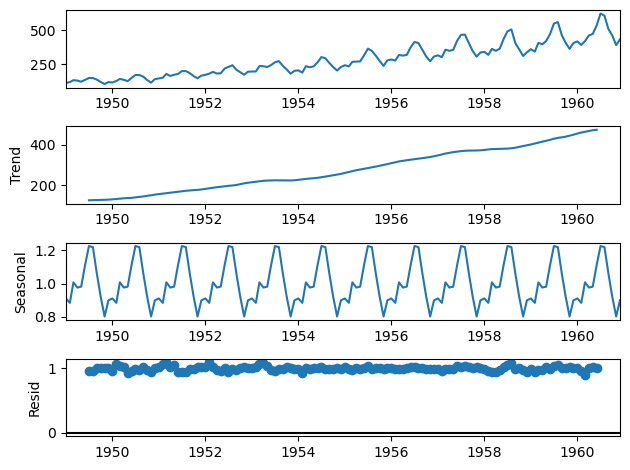

import warnings
warnings.filterwarnings("ignore")

Autocorrelation

Autocorrelation in a time series refers to the degree of similarity or relationship between a data point and its past values at different time lags. It measures how dependent the current value of the series is on its previous values.

To understand autocorrelation, let’s consider an example of daily stock prices. If there is a positive autocorrelation, it means that when the stock price increases today, there is a higher likelihood that it will also increase tomorrow. Similarly, if there is a negative autocorrelation, an increase in today’s stock price indicates a higher chance of a decrease in the price tomorrow.

Autocorrelation is essentially a way to measure the pattern or persistence of the time series. It helps us identify if there are any predictable relationships between past and current values. By analyzing autocorrelation, we can gain insights into the underlying dynamics and dependencies within the data.

Stationarity

Stationarity in a time series refers to the property where the statistical properties of the data do not change over time. In simpler terms, it means that the data has a consistent pattern or behavior throughout its entire duration.

To understand stationarity, let’s consider an example. Imagine you have a time series of daily temperature measurements for a city. If the data is stationary, it implies that the statistical properties of the temperature, such as the mean (average) and variance (spread), remain constant over time. This means that the temperature fluctuations and patterns observed in the past will continue to occur in the future.

stationarity

On the other hand, if the time series is not stationary, it suggests that the statistical properties of the data change over time. For instance, if the average temperature increases over the years, or if the temperature fluctuations become larger or smaller, the data is non-stationary.

Stationarity is an essential concept in time series analysis because many forecasting techniques and models assume stationarity to make accurate predictions. When a time series is stationary, it allows us to apply mathematical and statistical tools that rely on consistent patterns and relationships in the data.

If a time series is found to be non-stationary, various techniques can be applied to make it stationary, such as differencing to remove trends, or transformations to stabilize the variance.

import numpy as np
import matplotlib.pyplot as plt
import os
import plotly.express as px
import plotly.io as pio
pio.templates.default = "plotly_white"
import timesynth as ts
import pandas as pd
np.random.seed()

helper functions…

def plot_time_series(time, values, label, legends=None):
    if legends is not None:
        assert len(legends)==len(values)
    if isinstance(values, list):
        series_dict = {"Time": time}
        for v, l in zip(values, legends):
            series_dict[l] = v
        plot_df = pd.DataFrame(series_dict)
        plot_df = pd.melt(plot_df,id_vars="Time", var_name="ts", value_name="Value")
    else:
        series_dict = {"Time": time, "Value": values, "ts":""}
        plot_df = pd.DataFrame(series_dict)
    
    if isinstance(values, list):
        fig = px.line(plot_df, x="Time", y="Value", line_dash="ts")
    else:
        fig = px.line(plot_df, x="Time", y="Value")
    fig.update_layout(
        autosize=False,
        width=900,
        height=500,
        title={'text': label, 'y':0.9, 'x':0.5, 'xanchor': 'center', 'yanchor': 'top'},
        titlefont={"size": 25},
        yaxis = dict(title_text="Value", titlefont=dict(size=12)),
        xaxis = dict(title_text="Time", titlefont=dict(size=12))
    )
    
    return fig
    
def generate_timeseries(signal, noise=None):
    time_sampler = ts.TimeSampler(stop_time=20)
    regular_time_samples = time_sampler.sample_regular_time(num_points=100)
    timeseries = ts.TimeSeries(signal_generator=signal, noise_generator=noise)
    samples, signals, errors = timeseries.sample(regular_time_samples)
    return samples, regular_time_samples, signals, errors

Generating synthetic time series

Let’s take a look at a few practical examples where we can generate a few time series using a set of fundamental building blocks. You can get creative and mix and match any of these components, or even add them together to generate a time series of arbitrary complexity.

White Noise

White noise can be understood as a random and unpredictable pattern of data points that do not exhibit any discernible trend or seasonality. It serves as a benchmark against which other patterns and relationships in the data can be evaluated.

It has a constant mean and variance, and each data point is independent of the others. White noise is important to identify and remove from time series data because it represents the random fluctuations that are not informative or useful for analysis.

time = np.arange(200)
values = np.random.randn(200) * 100
plot_time_series(time, values, "White Noise")

Red Noise

Red noise, also known as random walk or persistent noise, is a type of pattern or behavior often observed in time series data. In simple terms, red noise represents a situation where the data exhibits a persistent, gradual change or trend over time. It is characterized by a correlation between adjacent data points, meaning that the value of one data point is influenced by the value of the previous point.

Unlike white noise, which is completely random and uncorrelated, red noise shows a memory or dependence on past values. It can be found in various phenomena, such as stock market fluctuations, natural processes, or economic indicators, and understanding its presence is essential for accurate analysis and prediction in time series data.

The ‘redness’ is parameterized by correlation coefficient r, such that:

\[ \large{x_{j+1} = r \cdot x_j + (1 - r^2)^{1/2}} \]

where:

$w$ = sample from white noise distribution

First set the correlation coefficient…

r = 0.4

Then createn and plot the red noise

time = np.arange(200)
white_noise = np.random.randn(200) * 100
values = np.zeros(200)

for i, v in enumerate(white_noise):
    if i==0:
        values[i] = v
    else:
        values[i] = r * values[i-1] + np.sqrt((1 - r**2)) * v
        
plot_time_series(time, values, "Red Noise Process")

Cyclical (seasonal) signals

A common signal you see in time series are cyclical signals. You can introduce seasonality into your generated series in a few ways. Let’s see how we can use a sinusoidal function to create cyclicity.

Sinusoidal

Sinusoidal signal with an amplitude of 1.5 and frequency set to 0.25

signal_1 = ts.signals.Sinusoidal(amplitude=1.5, frequency=0.25)

A second sinusoidal signal with an amplitude of 1 and a frequency of 0. 5

signal_2 = ts.signals.Sinusoidal(amplitude=1, frequency=0.5)

Now we can generate the time series…

samples_1, regular_time_samples, signals_1, errors_1 = generate_timeseries(signal=signal_1)
samples_2, regular_time_samples, signals_2, errors_2 = generate_timeseries(signal=signal_2)

plot_time_series(regular_time_samples, 
                 [samples_1, samples_2], 
                 "Sinusoidal Waves", 
                 legends=["Amplitude = 1.5 | Frequency = 0.25", 
                          "Amplitude = 1 | Frequency = 0.5"])

PseudoPeriodic

This is like the Sinusoidal class, but the frequency and amplitude itself has some stochasticity.

signal = ts.signals.PseudoPeriodic(amplitude=1, frequency=0.25)
samples, regular_time_samples, signals, errors = generate_timeseries(signal=signal)

plot_time_series(regular_time_samples, samples, "Pseudo Periodic")

Autoregressive signals

In simple terms, they refer to a type of signal or time series where each data point is influenced by its previous values. In other words, the current value of the signal is determined by a linear combination of its past values, with each previous value weighted by a specific coefficient.

An AR signal with parameters 1.5 and -0.75

\[ \large{y_{(t)} = 1.5y_{(t-1)} - 0.75y_{(t-2)}} \]

signal = ts.signals.AutoRegressive(ar_param=[1.5, -0.75])
samples, regular_time_samples, signals, errors = generate_timeseries(signal=signal)
plot_time_series(regular_time_samples, samples, "Auto Regressive")

A standard Gaussian distribution is defined by two parameters

mean
standard deviation.

There are two ways the stationarity assumption can be broken:

a change in mean over time
a change in variance over time

# White Noise with standard deviation = 0.3

noise = ts.noise.GaussianNoise(std=0.3)
signal = ts.signals.Sinusoidal(amplitude=1, frequency=0.25)

sin_samples, reg_time_samples, _, _ = generate_timeseries(signal=signal, noise=noise)
trend = regular_time_samples * 0.4

ts = sin_samples + trend
plot_time_series(reg_time_samples, ts, "Sinusoidal with Trend and White Noise")

Heteroscedasticity refers to a statistical phenomenon where the variability of data points is not constant across the range of values of an independent variable. In simpler terms, it means that the spread or dispersion of the data points changes as the values of the independent variable change. For example, in a scatterplot, heteroscedasticity would be present if the width of the data points’ spread becomes wider or narrower as you move along the x-axis. Heteroscedasticity can affect statistical analysis and can lead to biased estimates or incorrect inferences. It is important to account for heteroscedasticity when analyzing data to ensure accurate results.

Acquiring and Processing Time Series Data

Acquiring and processing time series data involves gathering and manipulating data points collected over a period of time. Time series data typically includes a timestamp and a corresponding value, such as stock prices, temperature readings, or website traffic.

stationarity

Here’s a general overview of the steps involved in acquiring and processing time series data:

Data Acquisition:
- Identify the data source: Determine where the time series data is coming from, such as sensors, databases, APIs, or files.
- Access the data: Establish a connection to the data source and retrieve the relevant time series data. This may involve querying a database, making API requests, or reading files.
Data Cleaning and Preprocessing:
- Handle missing values: Check for missing data points and decide on a strategy for dealing with them, such as filling in the missing values or removing incomplete entries.
- Remove outliers: Identify and handle any outliers or erroneous data points that may affect the analysis or modeling.
- Handle data quality issues: Address any data quality issues like inconsistent formatting, incorrect units, or data inconsistencies.
- Normalize or scale data: Depending on the specific analysis or modeling task, you may need to normalize or scale the data to ensure it falls within a certain range or has a specific distribution.
Data Exploration and Visualization:
- Explore the data: Analyze the characteristics of the time series data, such as trends, seasonality, or correlations between variables.
- Visualize the data: Create plots and charts to gain insights into the data, such as line plots, histograms, scatter plots, or heatmaps. Visualization can help identify patterns, anomalies, or relationships within the time series data.
Time Series Analysis:
- Statistical analysis: Apply statistical techniques to extract meaningful information from the time series data, such as calculating descriptive statistics, identifying autocorrelation, or performing time series decomposition.
- Modeling and forecasting: Build mathematical models or employ machine learning algorithms to forecast future values or estimate unknown data points based on historical patterns. Popular methods include autoregressive integrated moving average (ARIMA), exponential smoothing (ETS), or deep learning approaches like recurrent neural networks (RNNs).
Data Storage and Retrieval:
- Store the processed data: Save the cleaned and preprocessed time series data in a suitable format, such as a database or file, for future use or analysis.
- Enable efficient retrieval: Organize the data in a way that allows for efficient querying and retrieval based on time ranges or other relevant parameters.

It’s important to note that the specific steps and techniques involved in acquiring and processing time series data can vary depending on the context and requirements of the analysis or application.

def smaller(a, b):
    if a < b:
        return a
    else:
        return b

smaller(5, 4)

def n_smaller(a, b):
    return a * (a < b) + b * (b <= a)

n_smaller(1, 4)